Wind speed and direction tutorial

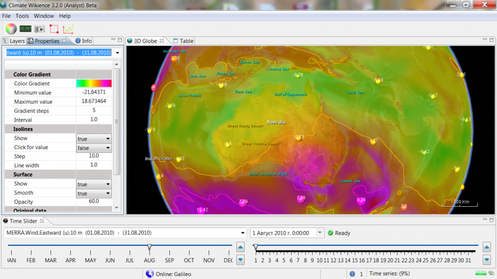
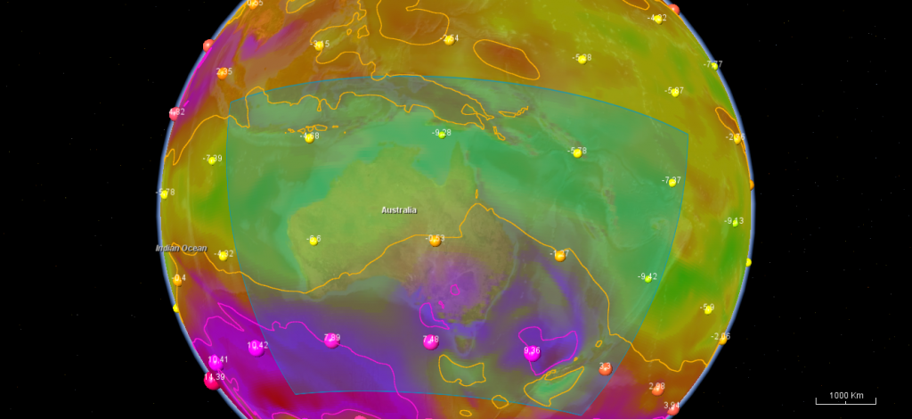
Originally, climate reanalysis data provide wind speed separately for Eastward (u) and Northward (v) directions. These are two different vectors.

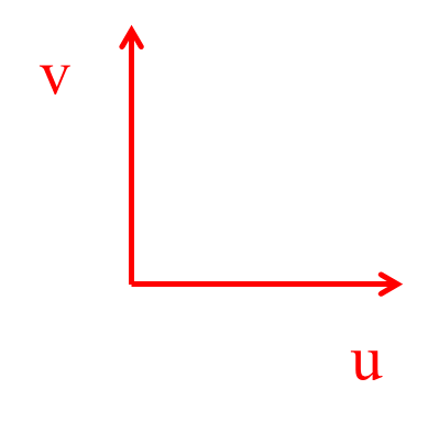
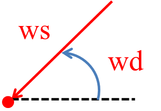
However, for most applications it is preferably to have wind speed (ws) and wind direction (wd) (azimuth) values instead.

This tutotial shows how to convert u-v vectors to wind speed and direction using RWikience. Wind speed and direction data exploratory tools are also introduced.

Prerequisite: you should have RWikience installed into R.
This RWikience introductory tutorial is also worth seeing.

Launch Climate Wikience. RWikience will be able to retrieve data only if Climate Wikience is currently running on your desktop.

Start your work by loading RWikience package and connecting to running Climate Wikience from R. Note: Climate Wikience should be running for successful connection.

# Load RWikience package
library(RWikience)
 
# Connect to Climate Wikience 
w<-WikienceConnect()

Time series retrieval consists of two parts.

1. Call “queryTimeSeries” with necessary parameters to prepare time series
2. Call other functions (find out number of points, retrieve time series for a selected point and other functions) to work with prepared time series

The next code retrieves (prepares) time series for

• Eastward wind speed at 10 meters altitude
• for each point in geographical region where
  • latitude south = -25,
  • longitude west = 130,
  • latitude north = -24,
  • longitude east = 131
• and time interval spans
  • since 1-st of January 1979 (inclusively)
  • to the 1-st of August 2014 (exclusively)

queryTimeSeries(w, "MERRA.Wind.Eastward (u).10 m", "01 01 1979", "01 08 2014", -25, 130, -24, 131)

NOTE: there are no limitations on time interval maximum length when you retrive time series using R unlike requesting time series in Climate Wikience.

You can copy/paste dataset name (i.e. MERRA.Wind.Eastward (u).10 m) from Climate Wikience (select the dataset in the tree on “Temporal layers” tab, the dataset name will appear in “Time Slider” drop-down list or “Properties” drop-down list)

Once the preparing operation finishes, you can check the number of points in the result (the output should be 6)

getTimeSeriesPointCount(w)

The coordinates of the resulting 6 points could be seen by calling

latlon <- getTimeSeriesPointsLatsLons(w)
latlon

The output should look like this:

lat      lon
1 -25.0 130.0000
2 -25.0 130.6667
3 -24.5 130.0000
4 -24.5 130.6667
5 -24.0 130.0000
6 -24.0 130.6667

Let’s take the first point in the result (it has coordinates lat = -25.0, lon = 130.0 ). Since data is hourly, there are 311904 values for the selected time interval

tU <- getTimeSeries(w, 0)
 
# See the first 10 values
tU[1:10,]
                  date     value
1  1979-01-01 00:00:00 -5.768760
2  1979-01-01 01:00:00 -4.866543
3  1979-01-01 02:00:00 -4.114307
4  1979-01-01 03:00:00 -3.606280
5  1979-01-01 04:00:00 -3.326102
6  1979-01-01 05:00:00 -3.213083
7  1979-01-01 06:00:00 -3.231349
8  1979-01-01 07:00:00 -3.344310
9  1979-01-01 08:00:00 -3.563092
10 1979-01-01 09:00:00 -3.926733

In this tutorial we will concentrate on the single location (point). We have u-vectors (tU) for this single point and now we will retrieve v-vectors (Northward wind speed component) for the same time interval and geographical region

queryTimeSeries(w, "MERRA.Wind.Northward (v).10 m", "01 01 1979", "01 08 2014", -25, 130, -24, 131)

Since query parameters are the same, the result contains time series for the same points. Thus, the first point will also have coordinates lat = -25.0, lon = 130.0. Now, get this first point from the result:

tV <- getTimeSeries(w, 0)
 
# Again, the first 10 rows are
tV[1:10, ]
                  date      value
1  1979-01-01 00:00:00 -1.2735988
2  1979-01-01 01:00:00 -1.2039323
3  1979-01-01 02:00:00 -0.8677690
4  1979-01-01 03:00:00 -0.5525676
5  1979-01-01 04:00:00 -0.2276626
6  1979-01-01 05:00:00  0.1847073
7  1979-01-01 06:00:00  0.6056390
8  1979-01-01 07:00:00  0.9443905
9  1979-01-01 08:00:00  1.1709728
10 1979-01-01 09:00:00  1.1513032

Now we have both u and v vectors for the point. Call the “convertUVtoSpeedAndDirection” function from RWikience package to obtain the data frame containing date, wind speed (ws) and wind direction (wd) columns.

Note: wind speed and direction values comply with the UK meteorological office standards. Wind direction is the azimuth (where FROM does the wind blow) as shown on the figure at the top of this tutorial (ws and wd).

result <- convertUVtoSpeedAndDirection(tU, tV)
 
# Check the first 10 rows
result[1:10, ]
                  date       ws        wd
1  1979-01-01 00:00:00 5.907677  77.55023
2  1979-01-01 01:00:00 5.013252  76.10461
3  1979-01-01 02:00:00 4.204824  78.09002
4  1979-01-01 03:00:00 3.648367  81.28868
5  1979-01-01 04:00:00 3.333884  86.08437
6  1979-01-01 05:00:00 3.218388  93.29008
7  1979-01-01 06:00:00 3.287615 100.61556
8  1979-01-01 07:00:00 3.475095 105.76900
9  1979-01-01 08:00:00 3.750574 108.19257
10 1979-01-01 09:00:00 4.092033 106.34094

The next section of the tutorial shows the use cases of EDA (Exploratory Data Analysis) that is possible with wind speed and direction time series for a single point (location). The result data frame is used as the parameter to the functions below.

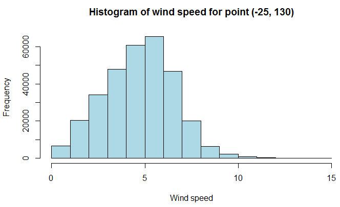
Histogram of wind speed for point (-25, 130) (latitude, longitude)

hist(result$ws, main = "Histogram of wind speed for point (-25, 130)", xlab = "Wind speed", col = "lightblue")

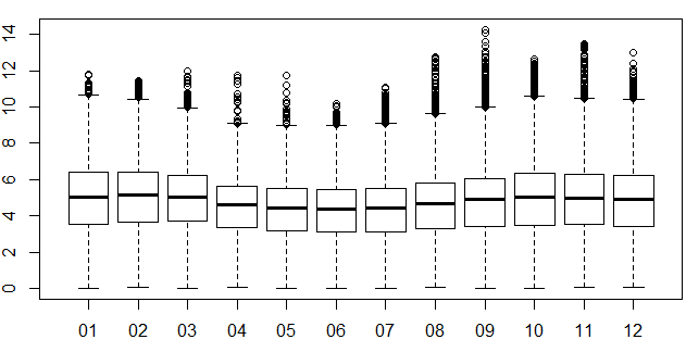
Monthly boxplot of wind speed

plot(as.factor(format(result$date, "%m")), result$ws)

OpenAIR package provides comprehensive tools to explore air pollution and wind data (see below).

library(openair)

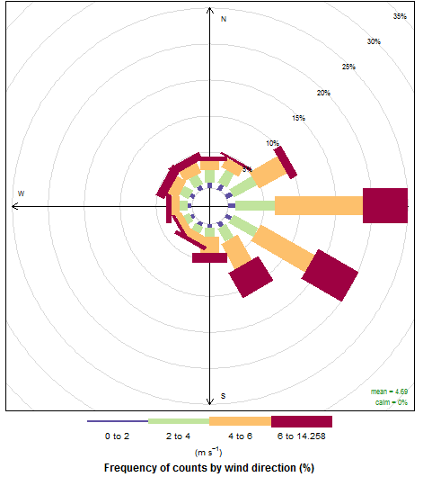
Wind rose shows the wind frequency from a particular direction. The data from the whole time interval are used

windRose(result)

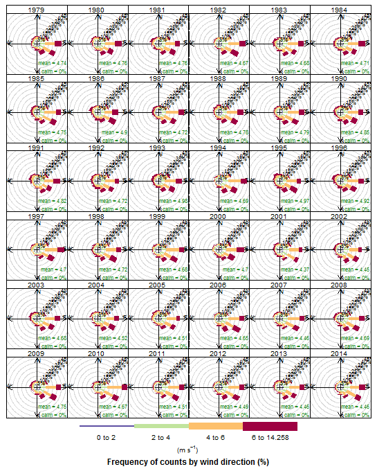
The same, but statistics is shown for each year separately

windRose(result, type = "year")

From OpenAir manual: “Each cell gives the total number of dates the wind was from that wind speed/direction. The number of dates is coded as a colour scale shown to the right. The scale itself is non-linear to help show the overall distribution.”

polarFreq(result)

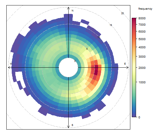
The same, but for a particular year

polarFreq(result, type = "year")

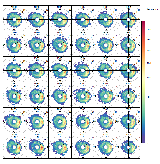
Display a calendar for a given year. In each cell of the calendar (each day) the wind direction is shown. The color of the cell is proportional to the wind speed. The longer the arrow, the greater wind speed is.

calendarPlot(result, pollutant = "ws", year = 1979, annotate = "ws")

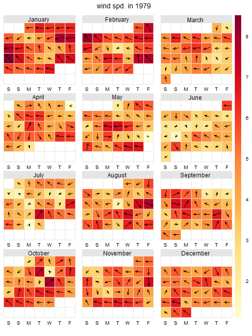
If you would like to use the wind speed and direction data somewhere else, save it to CSV file.

fileName = "D:/Wind_speed_25_130.csv"   # Path to file
write.csv(file = fileName, x = result)

You can download the R code used in this tutorial with a single file [wpdm_file id=13]

Related links

• RWikience package download
• RWikience: introduction tutorial
• Tutorial on retrieving time series in Climate Wikience (without R)

Email

Facebook

Google

Linkedin

Twitter

RWikience: introduction tutorial

All data in Climate Wikience are directly accessible from R using RWikience package

RWikience package allows to retrieve raster, time series data from Climate Wikience to R and also contains related utility fuctions. Steps to get data into R:

1. Download and install R from www.r-project.org/
2. Download and install an IDE like RStudio www.rstudio.com/ide/
3. Install rJava package (you will need this to run RWikience)
You can install rJava by typing the following code in R console:

install.packages(“rJava”)

4. Download RWikience package and install it into R

RWikience_path <- "path to where you downloaded RWikience package tar.gz"; install.packages(RWikience_path, repos = NULL, type = "source")   # Example (use "/" or "\\" in Windows): RWikience_path <- "C:/Users/User/WikienceFiles/RWikience_1.1-0.tar.gz" install.packages(RWikience_path, repos = NULL, type = "source")

5. Launch Climate Wikience (RWikience will work only when Climate Wikience is currently running)

The following two commands are required to start working with RWikience

# Load RWikience package
library(RWikience)
 
# Connect to running instance of Climate Wikience on your PC
w<-WikienceConnect()

To retrieve global maps (raster data), use getFloatMatrix function:

# Retrieve global matrix of NO2 concentration for 1-st of October 2004
m <- getFloatMatrix(w, "OMI.Nitrogen dioxide.ColumnAmountNO2TropCloudScreened", "01 10 2004")

To enable many other ways of processing data, convert the matrix to “raster” type of “raster” package:

# Load "raster" package
library(raster)
 
# Convert to R type "raster"
r <- convertToRaster(m)

Simply type “r” to view the properties of newly created raster:

> r
class       : RasterLayer 
dimensions  : 720, 1440, 1036800  (nrow, ncol, ncell)
resolution  : 0.25, 0.25  (x, y)
extent      : -180, 180, -90, 90  (xmin, xmax, ymin, ymax)
coord. ref. : +proj=longlat +datum=WGS84 
data source : in memory
names       : layer 
values      : -6.343879e+15, 4.233803e+16  (min, max)

Create 2-D map of the global NO2 distribution:

# Visualize raster
plot(r)

You can retrieve other maps in the same way:

m <- getFloatMatrix(w, "MERRA.Wind.Eastward (u).10 m", "01 08 2010")
r <- convertToRaster(m)
plot(r)
 
m <- getFloatMatrix(w, "Modis L3 Atmosphere.AEROSOL.LAND AND OCEAN.Optical Depth.Maximum", "04 08 2005")
r <- convertToRaster(m)
plot(r)

You can take a full dataset name to forward in to “getFloatMatrix” by simply activating it in Climate Wikience and copying its names from Time Slider drop-down box or Properties drop-down box.

R code used in this tutorial [wpdm_file id=7]

Email

Facebook

Google

Linkedin

Twitter

Tutorial on retrieving time series in Climate Wikience version 3.2

To retrieve time series in Climate Wikience, three steps should be taken to specify three necessary parameters:

1. Dataset (select in Layers/Temporal tab)
2. Geographical region on 3D globe (use “Region selector” tool)
3. Required time interval for which you would like the time series to be retrieved

Let’s cover these steps in detail.

1. Select dataset

Climate Wikience will retrieve time series for the current dataset. The current dataset is the dataset which properties are currently displayed on “Properties” tab. The name of the current dataset is also displayed on “Time slider” dropdown list:

You can make a dataset current in several ways:
• Find the dataset in tree view on “Layers/Temporal” tab and turn it on by checking the box left to the dataset name
• Select the dataset from dropdown list in “Properties” tab or “Time slider” if you have already turned it on some time earlier during your work with Climate Wikience

2. Select region

Press button “Select region” located on the toolbar. Climate Wikience will automatically “fly to” the geographical region for which time series are available. Use mouse to select the region. The available region on the 3D Globe will be colored blue.

2.1 Limitations on region size

Since there are thousands of grid points for which time series can be obtained, there is a limitation on the size of geographical region that can be selected (for which time series could be requested).

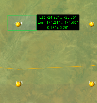
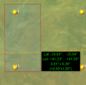
Each dataset has it own limitation on selected region size. To view the region size during selection and to keep the size in the allowed limits, turn on “Show cursor position” tool. When the region selection is disabled, this tool shows mouse cursor position (latitude and longitude). When the region selection is enabled, it shows the following region paramters near to mouse cursor:
• southern and northern latitude
• eastern and western longitudes
• region size (latitude degrees x longitude degrees)

When you are dragging mouse cursor and the size of the selected region is less than the maximum allowed for the current dataset, the region is colored green. When the region becomes oversized, it is colored red and additionally to region characteristics the size of the maximum allowed region appears:

In this case, the size of the maximum allowed region is 0.5°x1.0°. You can still select the region that is larger than the maximum allowed, however it will be automatically trimmed (shown below at time series request dialog).

2.2 Trimming of the selected region

Once you finished selecting the region, press on the toolbar. Time series request dialog will appear.

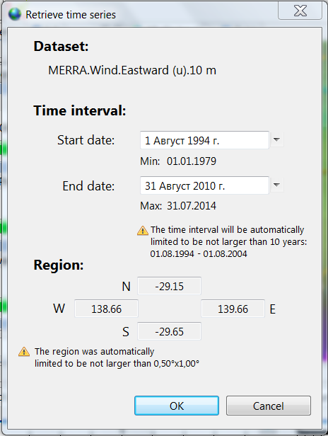
This dialog summarises the request by showing the selected dataset name, time interval and geographical region.

If you selected the region larger than maximum allowed, the corresponding notification will appear with warning icon . The oversized region will be automatically reduced to fit into the maximum allowed boundaries. The northern latitude and western longitude will remain the same (as you selected) while the southern latitude and eastern longitude of the region border will be changed.

In the dialog shown above, the difference between latitudes does not exceed 0.5° and between longitudes does not exceed 1°. The southern latitude was calculated by subtracting 0.5° from the value of nothern latitude. The eastern longitude was calculated by adding 1° to the western longitude.

3. Select time interval

The time series dialog allows to specify the time interval for which time series should be retrieved. There are two important notices about selecting time interval.

3.1 Available time interval

The available time interval for time series (shown at time series request dialog) may differ from the available time interval for gridded global dataset (shown on time slider)

For example, NASA MERRA wind speed gridded data are available globally currently only for August 2010, but time series for this dataset are available for Australia since 01 January till 31 July 2014 (35.5 years).

3.2 Limitations on the selected time interval length

Each dataset has limitation on the time interval length that could be requested per single query.

Select start and end date for time interval for which you would like to retrieve time series. If the selected time interval will exceed the maximum allowed length for current dataset, corresponding notification will appear. This notification will contain the maximum allowed time interval length and the reduced time interval for which time series will be requested.

In the reduced time interval, the starting date will be the same as you selected while the end date will be set to the earlier date than you selected to keep the interval length within maximum allowed. For example, if the maximum allowed time interval is 10 years, the end date is calculated as start date + 10 years.

The limit on time interval is introduced since there are datasets with hourly time steps and long available time periods. For example, NASA MERRA wind speed and direction data are avaialbe for 35.5 years with hourly time step. This is approximately 311000 values for a single grid point.

Results

When you selected all parameters, press the OK button on time series request dialog. Climate Wikience will send your request to server. Please, wait while the server will extract the data. Once Climate Wikience receives the data, it prepares the interface to display the result. If the resulting time series has thousands of values, the process may take some time to complete, so you will be notified by the progress bar.

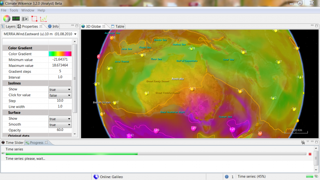
Time series are visualized by data table.

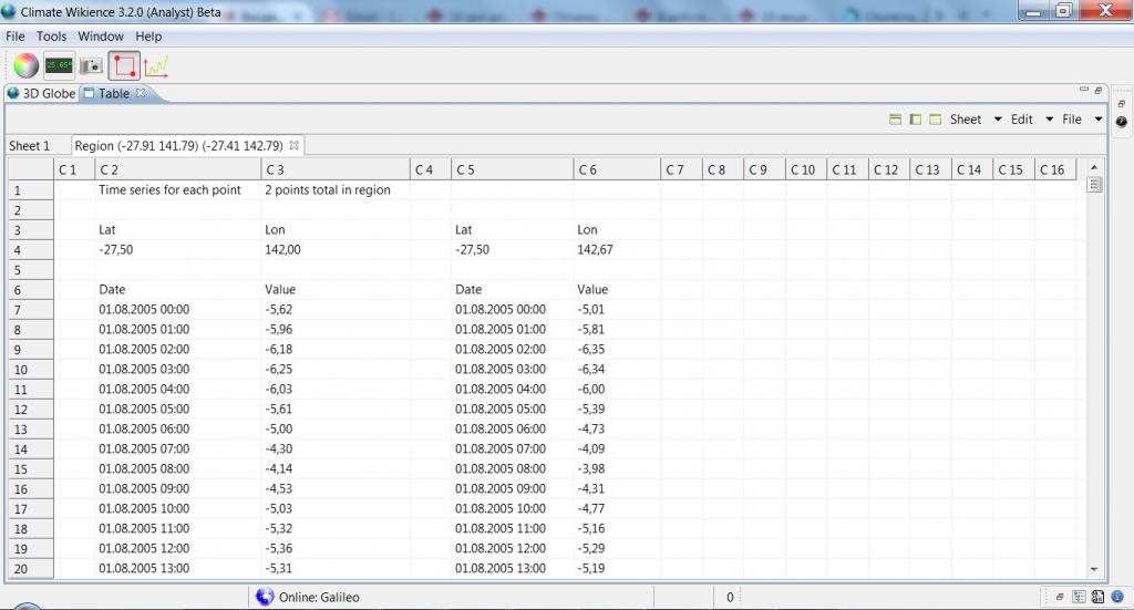
The format of the time series in data table is as follows. The tab name of the data table contains the cordinates of the selected region. In case if region was reduced, the coordinates of the reduced region are shown. At the top of the data table sheet, there is the number of points covered by the region (maybe reduced).

For each grid point of the region, its coordinates are shown (Lat and Lon). Other rows of the data table sheet show the dates and the values of the time series for a grid point (one row per one date).

If you would like to select time series for different time interval but for the same region (since there is a limitation on the maximum time interval length per single query), do not select region again. Instead, call the time series request dialog by clicking on the toolbar. The dialog will contain both the old region and the old time interval you used for your previous query. Adjust time interval as you need and press OK button. Climate Wikience will retrieve time series for the same region as previous query but for updated time interval.

If you would like to save the resulting time series as CSV or Excel file, use corresponding buttons at the top right corner of the data table.

Related links

• Retrieve time series from Climate Wikience to R

Email

Facebook

Google

Linkedin

Twitter